[This is an updated version of this post with improved functions and a reproducible example]

I really like the package Gviz to prepare figures for presentations and publications (I have used in B plus some tidying up in inskape). It is a fantastic visualization package, but the time and effort that it takes to get the figures just right is a little too much for my daily. An example of this is when plotting coverage tracks; by default axis of each panel are scaled independently which makes visualization tricky.

Let’s fist load the packages. derfinder contains some example datasets (chosen almost randomly). You can find the vignette here.

library('Gviz')
library('rtracklayer')
library('derfinderData')
files <- dir(system.file('extdata', 'A1C', package = 'derfinderData'),  full.names = TRUE)
names(files) <- gsub('\\.bw', '', dir(system.file('extdata', 'AMY', package = 'derfinderData')))
head(files)

##                                                                                 HSB113 
## "/home/adomingu/R/x86_64-pc-linux-gnu-library/3.3/derfinderData/extdata/A1C/HSB103.bw" 
##                                                                                 HSB123 
## "/home/adomingu/R/x86_64-pc-linux-gnu-library/3.3/derfinderData/extdata/A1C/HSB114.bw" 
##                                                                                 HSB126 
## "/home/adomingu/R/x86_64-pc-linux-gnu-library/3.3/derfinderData/extdata/A1C/HSB123.bw" 
##                                                                                 HSB130 
## "/home/adomingu/R/x86_64-pc-linux-gnu-library/3.3/derfinderData/extdata/A1C/HSB126.bw" 
##                                                                                 HSB135 
## "/home/adomingu/R/x86_64-pc-linux-gnu-library/3.3/derfinderData/extdata/A1C/HSB130.bw" 
##                                                                                 HSB136 
## "/home/adomingu/R/x86_64-pc-linux-gnu-library/3.3/derfinderData/extdata/A1C/HSB135.bw"

bw_file1 <- files[1]
bw_file2 <- files[3]
bw1 <- import(files[1])
bw2 <- import(files[2])

Let’s create some genomic regions to look at:

gr1 <- GRanges(
  seqnames=c("chr21", "chr21"),
  ranges=IRanges(c(48055507, 17059283), c(48085155, 17070283)),
  strand=c("+", "-")
  )
gr1

## GRanges object with 2 ranges and 0 metadata columns:
##       seqnames               ranges strand
##          <Rle>            <IRanges>  <Rle>
##   [1]    chr21 [48055507, 48085155]      +
##   [2]    chr21 [17059283, 17070283]      -
##   -------
##   seqinfo: 1 sequence from an unspecified genome; no seqlengths

One of these is the gene PRMT2, and the other is some random region without an annotated gene. We will see it’s usefulness later.

And does the plot look like using the defaults? Let’s have a look:

gen = "hg19"
gr1a <- as.data.frame(gr1)
start=gr1a[1,2]
end=gr1a[1,3]

gTrack <- BiomartGeneRegionTrack(
  genome = gen,
  chromosome = "chr21",
  start = start,
  end = end,
  name = "ENSEMBL")

dTrack1 <- DataTrack(
  bw_file1,
  type = "l",
  name="track1")
dTrack2 <- DataTrack(
  bw_file2,
  type = "l",
  name="track2")

# call the display function plotTracks
track.list=list(dTrack1, dTrack2, gTrack)
plotTracks(track.list,from=start,to=end,chromsome="chr21")

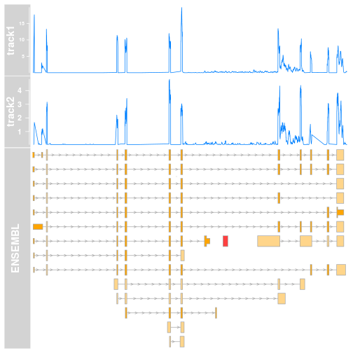
Two things become clear, though not immediately:

• the coverage is lower in track2, but since these tracks do not share the same scale a simple glance would convey the wrong message.
• Due to the internals of Gviz, the y-axis of both tracks have different front size. This is because they are scaled to the y-max. This could be fixed, but makes the figure a bit clunky for presentations.

The way I am solving both these issues is to determine the maximal coverage for both tracks, and then adjust the y-lim of both to this value. Initially I was doing this manually, using a Kent tool in the terminal, and using the value in R. This is of course time consuming and not adequate if one starts using Gviz on a regular basis, mixing and matching tracks in the plots.

Because I had a project that required me to plot the coverage over an entire chomosome rather than a gene, my first programatic solution was to calculate the top coverage for a given chromosome. The basic function maxCovBw will take an imported BigWig and do this. The maxCovFiles function is a wrapper that will do the same but for a list of files.

## calculate the max values
 maxCovBw <- function(gr, myChr) {
    max_cov <- max(gr[seqnames(gr) %in% myChr,]$score)
    return(max_cov)
 }

 maxCovFiles <- function(bws, chrs){
    for(i in seq_along(chrs)){
       myChr = chrs[i]
       print(myChr)
       max_coverage <- c()
       max_cov <- round(
          max(
             sapply(bws, maxCovBw, myChr=myChr)
          )
       , 0)
       max_coverage[myChr] <- max_cov 
    }
    return(data.frame(max_coverage))
 }

max_cov <- maxCovFiles(list(bw1, bw2), seqnames(seqinfo(bw1)))

## [1] "chr21"

We can see that there is only one chromosome in these files:

seqnames(seqinfo(bw1))

## [1] "chr21"

seqnames(seqinfo(bw2))

## [1] "chr21"

which we can now use to call the function:

max_cov <- maxCovFiles(list(bw1, bw2), "chr21")

## [1] "chr21"

max_cov

##       max_coverage
## chr21         2250

As I mentioned, this is useful for those situations when I am plotting a full chromosome, but in most situations what is being plotted is a narrow region, for instance, at a gene. Also a chromosome could be represented as a region as c(0, seqlengths(seqinfo(bw1)). So let’s modify the function:

## calculate the max values
maxCovBw <- function(bw, gr) {
  ovlp <- subsetByOverlaps(bw, gr)
  if (length(ovlp) > 0) {
    print('not empty')
    max_cov <- max(ovlp$score)
  } else {
    print('WARNING: The selected genomic region has no coverage value in the BigWig')
    print('WARNING: Coverage value is arbitrary set to Zero.')
    max_cov <- 0 
  }
  print(max_cov)
  return(max_cov)
}

maxCovFiles <- function(bws, gr){
  # bws <- lapply(bws, rtracklayer:::import)
  max_cov <- c()
  for(i in 1:length(gr)){
    my_feat = gr[i, ]
    max_cov[i] <- round(
      max(
        sapply(bws, maxCovBw, gr=my_feat)
      )
      , 2)
  }
  values(gr) <- max_cov 
  return(gr)
}


gr2 <- maxCovFiles(list(bw1, bw2), gr1)

## [1] "not empty"
## [1] 19.84
## [1] "not empty"
## [1] 10.06
## [1] "WARNING: The selected genomic region has no coverage value in the BigWig"
## [1] "WARNING: Coverage value is arbitrary set to Zero."
## [1] 0
## [1] "WARNING: The selected genomic region has no coverage value in the BigWig"
## [1] "WARNING: Coverage value is arbitrary set to Zero."
## [1] 0

gr2

## GRanges object with 2 ranges and 1 metadata column:
##       seqnames               ranges strand |         X
##          <Rle>            <IRanges>  <Rle> | <numeric>
##   [1]    chr21 [48055507, 48085155]      + |     19.84
##   [2]    chr21 [17059283, 17070283]      - |         0
##   -------
##   seqinfo: 1 sequence from an unspecified genome; no seqlengths

As you can see we now have the top value (which is pretty low) for each of our regions of interest. The coordinates selected contain an edge case for which there is no overlap. I decided to set it to zero to avoid breaking things. How does this look like in a plot then?

gr2 <- as.data.frame(gr2)
start=gr2[1,2]
end=gr2[1,3]

gTrack <- BiomartGeneRegionTrack(
  genome = gen,
  chromosome = "chr21",
  start = start,
  end = end,
  name = "ENSEMBL")

max_cov=gr2[1,6]

dTrack1 <- DataTrack(
  bw1,
  type = "l",
  ylim=c(0, max_cov),
  name="track1")
dTrack2 <- DataTrack(
  bw2,
  type = "l",
  ylim=c(0, max_cov),
  name="track2")

# call the display function plotTracks
track.list=list(dTrack1, dTrack2, gTrack)
plotTracks(track.list,from=start,to=end,chromsome="chr21")

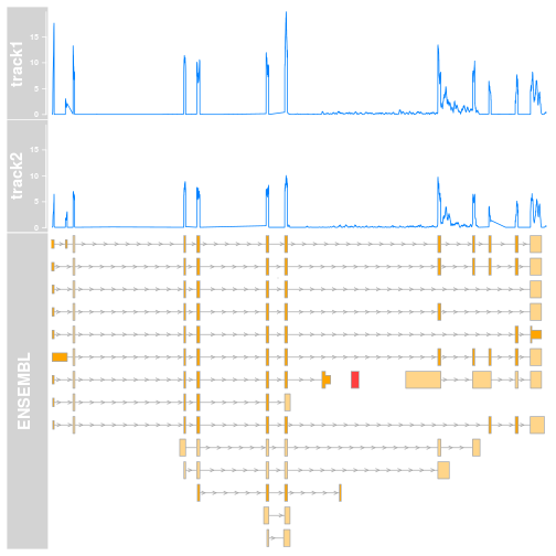
This simple change, ylim=c(0, max_cov), makes massive visual difference. A quick look at the plot and it will immediately be clear that track1 has higher coverage, and the visuals are now more consistent. This is something that could go into a manuscript draft without too many changes.

Of course both functions could do with some more input testing and cleaning up, but they are working and a good starting point for a quick plot. One thing that is missing and would be useful is the ability use bam/sam as an input as BigWigs would become limiting in certain situations. Something to improve once the need arises.